My sample Jupyter Notebook
In [1]:
import sys
sys.version_info
sys.version_info(major=3, minor=6, micro=2, releaselevel='final', serial=0)
In [2]:
%matplotlib inline
import matplotlib.pyplot as plt
import numpy as np
In [3]:
x = np.linspace(0, 3*np.pi, 500)
plt.plot(x, np.sin(x**2))
plt.title('A simple chirp');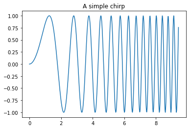
Setting up files for Jekyll
From the command line:
jupyter nbconvert --to markdown <notebook>.ipynb --config jekyll.py
Now some LaTeX magic:
\[E = m c^2\]Be aware that this is a markdown cell inside a Jupyter notebook, and the formula is converted by Jupyter.
Experiments
In [4]:
import math
import numpy as np
import tables as pt
from IPython.display import display, Math, Latex, SVG
The wing
In [5]:
c_r = 4.0; c_t = 1.5; b = 27; Lambda_le = 25*math.pi/180In [6]:
Latex(
    r'\begin{array}{rl}'
    +  r'\text{root chord,}\, c_{\mathrm{r}}: & ' + r'{0}'.format(c_r) + r'\,\text{m}'
    +  r'\newline'
    +  r'\text{tip chord,}\, c_{\mathrm{t}}: & ' + r'{0}'.format(c_t) + r'\,\text{m}'
    +  r'\newline'
    +  r'\text{span,}\, b: & ' + r'{0}'.format(b) + r'\,\text{m}'
    +  r'\newline'
    +  r'\text{leading edge sweep,}\, \Lambda_{\mathrm{le}}: &'
    +    r'{0}'.format(Lambda_le*180/math.pi) + r'\,\text{deg}'
    +r'\end{array}'
)
\begin{array}{rl}\text{root chord,}\, c_{\mathrm{r}}: & 4.0\,\text{m}\newline\text{tip chord,}\, c_{\mathrm{t}}: & 1.5\,\text{m}\newline\text{span,}\, b: & 27\,\text{m}\newline\text{leading edge sweep,}\, \Lambda_{\mathrm{le}}: &25.0\,\text{deg}\end{array}
Testing tikz output in Jupyter notebooks
In [7]:
%load_ext tikzmagicThen start each cell with the magic string: %%tikz followed by optional
directives.
Directives:
-s, --size: Pixel size of plots.
            example: -s <width,height>. Default is -s 400,240

-f, --format: Plot format (png, svg or jpg)

-l, --library: TikZ libraries to load, separated by comma.
            example: -l matrix,arrows.

-S, --save: Save a copy to "filename".

-p, --package: LaTeX packages to load, separated by comma.
            example: -p pgfplots,textcomp

-e, --encoding: text encoding.
            example: -e utf-8
In [8]:
%%tikz --scale 2 --size 300,300 -f svg
\draw (0,0) rectangle (1,1);
\filldraw (0.5,0.5) circle (.1);
In [9]:
%%tikz -p pgfplots -f svg
\begin{axis}[
  xlabel=$x$,
  ylabel={$f(x) = x^2 - x +4$}
]
\addplot {x^2 - x +4};
\end{axis}
In [10]:
%%tikz -p pgfplots -f svg -l calc,positioning
\path node[fill=red](ROW_1){this is some line of text};
\path node
[   fill=green,
    above=0mm of ROW_1.north west,
    xshift=-5mm,
    anchor=south west,
    scale=0.5
] (lt) {little tag};

\path node
[   fill=green,
    above left=0mm and 5mm of lt.north west,
    anchor=south west,
    scale=0.5
]{little tag};
In [11]:
%%tikz -p tkz-fct -l positioning -f svg -s 800,500

\begin{scope}
\tkzInit[xmin=-3,xmax=3,xstep=2, ymin=-3,ymax=3,ystep=2]
\tkzGrid[sub,subxstep=1,subystep=1](-2,-2)(2,2)
\tkzAxeXY
\node (a) at (3,0) {hello};
\end{scope}

\begin{scope}[xshift=5cm]
\tkzInit[xmin=-3,xmax=3,xstep=2, ymin=-3,ymax=3,ystep=2]
\tkzGrid[sub,subxstep=1,subystep=1](-2,-2)(2,2)
\tkzAxeXY
\node (b) at (3,0) {hello};
\tkzText[above,color=red](3,0){hello}
\end{scope}
In [12]:
%%tikz -l decorations.pathreplacing,shapes.misc -f svg -s 800,500

\tikzset{
    show curve controls/.style={
        decoration={
            show path construction,
            curveto code={
                \draw [blue, densely dashed]
                    (\tikzinputsegmentfirst) -- (\tikzinputsegmentsupporta)
                    node [at end, cross out, draw, solid, red, inner sep=2pt]{};
                \draw [blue, densely dashed]
                    (\tikzinputsegmentsupportb) -- (\tikzinputsegmentlast)
                    node [at start, cross out, draw, solid, red, inner sep=2pt]{};
            }
        }, decorate
    }
}

\draw [gray!50]  (0,0) -- (1,1) -- (3,1) -- (1,0)  -- (2,-1) -- cycle;
\draw [show curve controls] plot [smooth cycle] coordinates {(0,0) (1,1) (3,1) (1,0) (2,-1)};
\draw [red] plot [smooth cycle] coordinates {(0,0) (1,1) (3,1) (1,0) (2,-1)};

\draw [gray!50, xshift=4cm]  (0,0) -- (1,1) -- (3,-1) -- (5,1) -- (7,-2);
\draw [cyan, xshift=4cm, line width=1.2pt] plot [smooth, tension=2] coordinates { (0,0) (1,1) (3,-1) (5,1) (7,-2)};
\draw [show curve controls,cyan, xshift=4cm] plot [smooth, tension=2] coordinates { (0,0) (1,1) (3,-1) (5,1) (7,-2)};