International Standard Atmosphere (ISA)
The knowledge of standard atmosphere is required for producing pressure instruments, performing data reductions of flight tests, and pronouncing certain safety regulations for the aircraft.
The physical characteristics of the atmosphere are not steady and constant but change with altitude, location (longitude and latitude) on the globe, season, and time of the day, and with the solar sunspot activity. The performance of an aircraft depends on the physical characteristics of the atmospheric air through which it flies. The performance data of an aircraft or comparison of the performance of different aircraft have meaning only if they are considered with respect to some commonly agreed upon reference atmosphere. This reference atmosphere is usually the standard atmosphere, where the temperature, pressure, and density vary with altitude only. The fixation of standard atmosphere allows for the design of instruments for measuring altitude and airspeed. The pressure altitude, temperature altitude, and density altitude have meaning only after the standard atmosphere has been specified.
It is presently possible to specify the prevailing atmospheric conditions up to an altitude of 2000 km at any latitude and longitude of our globe. If desired, each country can have its own standard atmosphere. For general aviation purposes it is pertinent to develop internationally known reference atmosphere. Several reference atmospheric models have been established.
A number of standard versions exist: NACA’s atmosphere (1955), the ARDC (1959), the US standard (1962, amended in 1976) and the ICAO standard. These models, available in tabular form, are basically equivalent to each other up to about 20 km (65000 ft), that covers most of the atmospheric flight mechanics. We shall be concerned with altitudes below 31 km, or about 100000 ft.
The ISA Thermodynamic model
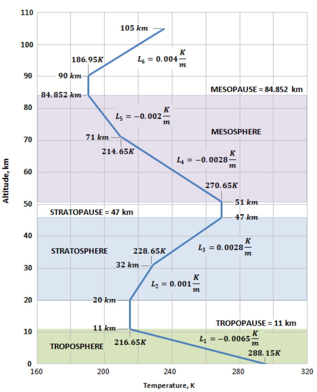
Air temperature distribution with altitude is the most important characteristic as it also determines the other elements of the atmosphere model. In a standard atmosphere, the temperature distribution is obtained by making several measurements at different altitudes. The temperature distribution of the U.S. standard atmosphere 1976, is presented in the figure below up to an altitude of 105 km.
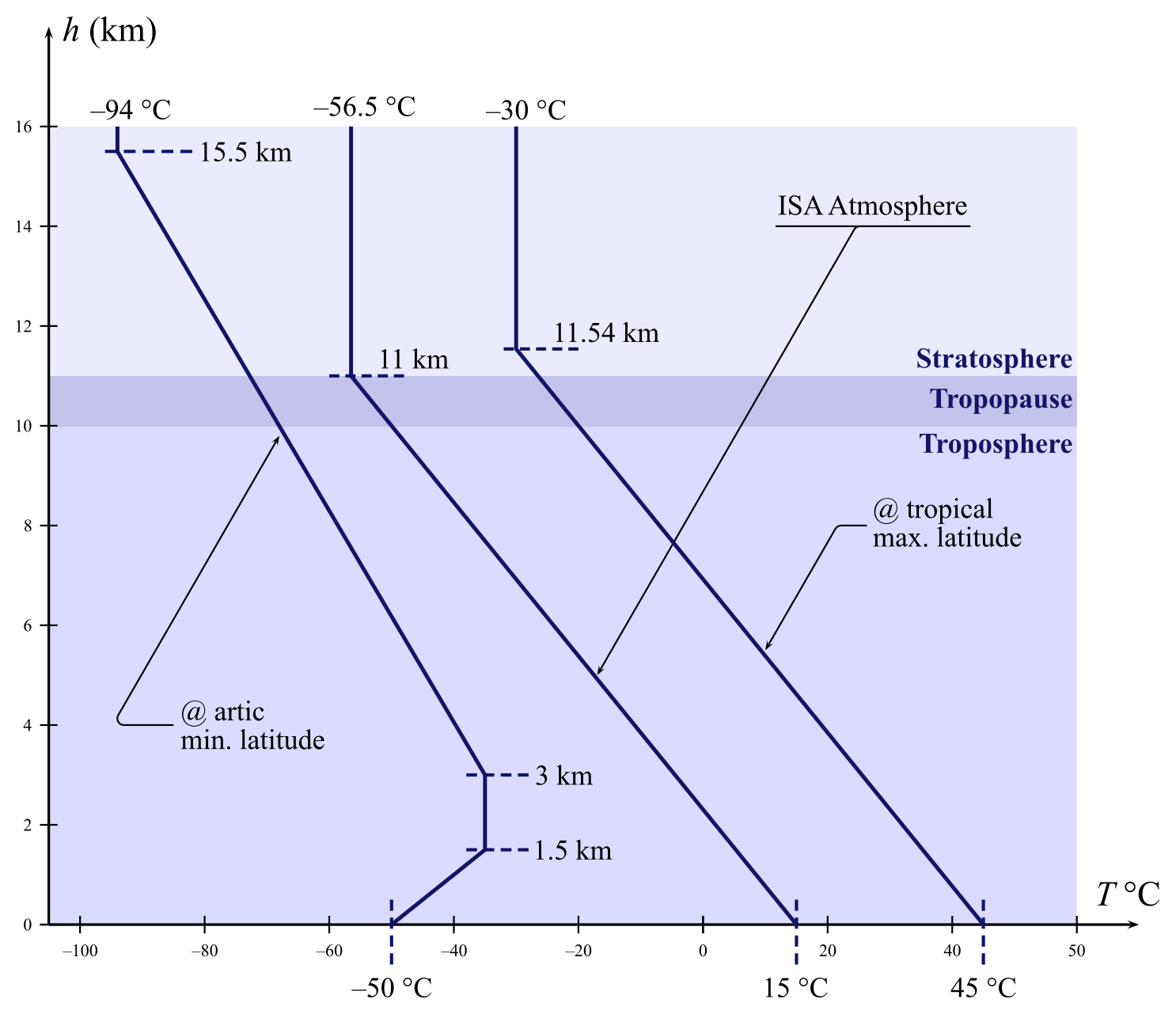
Next figure reports the ISA temperature up to 16 km with two variations of the model better suited for tropical and artic latitudes.
The temperature distribution in the standard atmosphere consists of mostly straight lines, each one characterized by a constant lapse rate
\begin{equation} \lambda = - \mathrm{d}T / \mathrm{d}h \label{eq:ISA:Lapse:Rate} \end{equation}
Thus, the atmosphere has either isothermal regions of zero lapse rate, or constant gradient regions of positive or negative lapse rates. The lapse rate $\lambda$ is positive in troposphere and mesosphere. The isothermal regions in the above figures are: 1) from 11.1 km to 20 km, 2) from 47.4 km to 51 km, and 3) from 86 km to 91 km.
Having obtained the temperature variation empirically, the pressure and density variations are calculated from the laws of hydrostatics and from the equation of state by assuming that the medium of air is continuum, perfect gas, and at rest. The variations of pressure and density with altitude can then be expressed analytically.
By the perfect gas hypothesis the local air pressure is given by the equation of state
\begin{equation} p = \rho \, R\, T \label{eq:Air:Perfect:Gas} \end{equation}
where $\rho$ is the density, $T$ is the temperature, and $R = 287\,\mathrm{J}/(\mathrm{kg}\,{}^\circ\mathrm{K})$ is the air constant. Moreover, the local speed of sound $a$ is given by the equation
\begin{equation} a = \sqrt{\strut \,\gamma \, R \, T \, } \label{eq:Air:Perfect:Gas:Sound} \end{equation}
where $\gamma = 1.4$ is the air specific heat ratio.
It can be shown that a small difference in altitude $\mathrm{d}h$ corresponds to a vertical difference in static pressure $\mathrm{d}p$ such that
\begin{equation} \frac{\mathrm{d}p}{p} = - g_0 \, \frac{\mathrm{d}h}{R \, T} \label{eq:Air:Stevino:Pressure} \end{equation}
where $g_0 = 9.807\,\mathrm{m/s}^2$ is the gravity acceleration at sea level (assumed constant throughout the atmosphere). The above equation is known as the law of Stevino that, combined with the definition of lapse rate, $-\lambda\, \mathrm{d}h = \mathrm{d}T$, yields
\begin{equation} \frac{\mathrm{d}p}{p} = \frac{g_0}{\lambda \, R} \,\frac{\mathrm{d}T}{T} \label{eq:Air:Stevino:Temperature} \end{equation}
This formula is valid throughout the atmosphere if the lapse rate is modelled as a function of altitude. In particular, according to the ISA model, $\lambda(h)$ assumes different constant values in different altitude intervals (i.e. those corresponding to Troposphere, Tropopause, Low and High Stratosphere, etc.). The integrating of (\ref{eq:Air:Stevino:Temperature}) between two altitudes $h_1 < h_2$ belonging to one of these constant-lapse-rate intervals, assuming $p_1=p(h_1)$, $p_2=p(h_2)$, $T_1=T(h_1)$, $T_2=T(h_2)$, yields \begin{equation} \int_{p_1}^{p_2} \frac{\mathrm{d}p}{p} = \frac{g_0}{\lambda \, R} \, \int_{T_1}^{T_2} \frac{\mathrm{d}T}{T} \quad \Longrightarrow \quad \ln \left( \frac{p_2}{p_1} \right) = \frac{g_0}{\lambda \, R} \, \ln \left( \frac{T_2}{T_1} \right) \label{eq:Air:Stevino:Integration:A} \end{equation}
The above result can be rearranged as follows:
\begin{equation} \frac{p_2}{p_1} = \left( \frac{T_2}{T_1} \right)^{g_0/(\lambda \, R)} \quad \Longrightarrow \quad \frac{\rho_2}{\rho_1} = \frac{p_2}{R\,T_2} \frac{R\,T_1}{p_1} = \left( \frac{T_2}{T_1} \right)^{[\,g_0/(\lambda \, R)\,] - 1} \label{eq:Air:Stevino:Integration:B} \end{equation}
The ratios (\ref{eq:Air:Stevino:Integration:B}) can be rewritten assuming ‘1’$\rightarrow\mathrm{SL}$ and ‘2’$\rightarrow h \le 11\,\mathrm{km}$, and substituting the ISA numeric values of air properties at sea level (SL)
- $\rho_\mathrm{SL} = 1.225\,\mathrm{kg}/\mathrm{m}^3$
- $p_\mathrm{SL} = 1.0133\cdot 10^5 \,\mathrm{N}/\mathrm{m}^2$
- $T_\mathrm{SL} = 15.15\,{}^\circ\mathrm{C} = 288.15\,{}^\circ\mathrm{K}$
- $a_\mathrm{SL} = 340.294\,\mathrm{m/s}$
Hence the following nondimensional ratios are introduced:
\begin{equation} \sigma = \frac{\rho}{\rho_\mathrm{SL}}\,,\;\; \delta = \frac{p}{p_\mathrm{SL}}\,,\;\; \Theta = \frac{T}{T_\mathrm{SL}}\,,\;\; \bar{a} = \frac{a}{a_\mathrm{SL}} \label{eq:ISA:Ratios} \end{equation}
named relative density, relative pressure, relative temperature, and relative speed of sound, respectively.
These are plotted in the next figure.
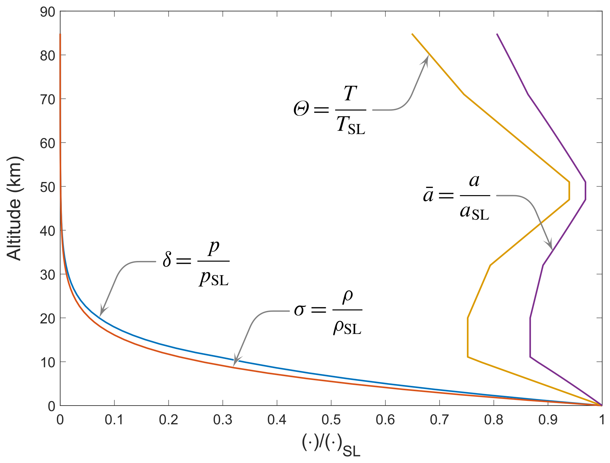
When the above graph is entered with the abscissa $p/p_\mathrm{SL}$, for instance by knowing the external pressure $p$ in flight, and the corresponding $h$ is read on the $Y$-axis from the $\delta$-curve, the resulting value is called pressure-altitude. If the local temperature is known and the graph is entered with the ratio $T/T_\mathrm{SL}$ then the altitude resulting from the $\Theta$-curve is called temperature-altitude. When the same process is based on a known density value then the resulting altitude is called density-altitude. For example, a pressure $p = 54019\,\mathrm{N}/\mathrm{m}^2$, i.e. a relative pressure $\delta = 0.533$, yields a pressure-altitude of $5000\,\mathrm{m}$.
In the troposphere, where the temperature law is
\begin{equation} T(h) = T_\mathrm{SL} - \lambda_0 \, h \label{eq:ISA:Temperature:Troposphere} \end{equation}
with $\lambda_0 = 0.0065\,{}^\circ\mathrm{C/m}$, given the SL values reported above, formulas (\ref{eq:Air:Stevino:Integration:B}) become:
\begin{equation} \delta (h) = \left( \frac{T(h)}{T_\mathrm{SL}} \right)^{\frac{g_0}{\lambda_0 R}} = \left( \frac{T(h)}{T_\mathrm{SL}} \right)^{\color{blue}{5.256}} \label{eq:ISA:Ratios:Troposphere:Delta} \end{equation}
\begin{equation} \sigma (h) = \left( \frac{T(h)}{T_\mathrm{SL}} \right)^{\frac{g_0}{\lambda_0 R} - 1} = \left( \frac{T(h)}{T_\mathrm{SL}} \right)^{\color{blue}{4.256}} \label{eq:ISA:Ratios:Troposphere:Sigma} \end{equation}