Note
This page was generated from a Jupyter notebook.
pathsim-flight: JSBSim as a PathSim Block
pathsim-flight bridges JSBSim and PathSim. It provides:
Class |
Description |
|---|---|
|
Wraps a JSBSim FDM as a discrete-time PathSim |
|
International Standard Atmosphere model: given geometric altitude and temperature offset, returns pressure, density, temperature, and speed of sound. |
Airspeed utilities |
|
Install
pip install pathsim
pip install git+https://github.com/pathsim/pathsim-flight.git
1. Imports
[1]:
import numpy as np
import matplotlib
import matplotlib.pyplot as plt

import jsbsim
import pathsim
import pathsim_flight

from pathsim import Simulation, Connection
from pathsim.blocks import Scope, Constant
from pathsim_flight import JSBSimWrapper, ISAtmosphere
from pathsim_flight.utils.airspeed_conversions import CAStoTAS, TAStoCAS

matplotlib.rcParams.update({'figure.dpi': 120, 'axes.grid': True, 'grid.alpha': 0.4})

# Suppress JSBSim console output globally
# jsbsim.FGJSBBase().debug_lvl = 0

print(f"JSBSim version        : {jsbsim.__version__}")
print(f"PathSim version       : {pathsim.__version__}")
print(f"pathsim-flight version: {pathsim_flight.__version__}")
JSBSim version        : 1.3.1.dev1
PathSim version       : 0.20.0
pathsim-flight version: 0.1.2.dev1+g904cf68e8
2. International Standard Atmosphere
ISAtmosphere is a PathSim Function block. Its two inputs are:
Port 0 – geometric altitude [m]
Port 1 – temperature offset from ISA standard day [K] (0 = standard day)
Its four outputs are pressure [Pa], density [kg/m³], temperature [K], and speed of sound [m/s].
[2]:
from pathsim.blocks import Source

# Sweep altitude from 0 to 11 000 m (tropopause)
alt_max_m = 11_000.0
altitudes_m = np.linspace(0, alt_max_m, 200)

isa = ISAtmosphere()
temp_offset = Constant(0.0)   # standard day

# We will evaluate standalone (not in a Simulation) for a quick sweep
pressures   = []
densities   = []
temperatures = []
speeds_of_sound = []

for alt in altitudes_m:
    result = isa._eval(alt, 0.0)
    pressures.append(result[0])
    densities.append(result[1])
    temperatures.append(result[2])
    speeds_of_sound.append(result[3])

fig, axes = plt.subplots(2, 2, figsize=(12, 8))
fig.suptitle('International Standard Atmosphere', fontsize=14)

axes[0, 0].plot(pressures, altitudes_m / 1000, color='steelblue')
axes[0, 0].set_xlabel('Pressure [Pa]')
axes[0, 0].set_ylabel('Altitude [km]')
axes[0, 0].set_title('Pressure')

axes[0, 1].plot(densities, altitudes_m / 1000, color='darkorange')
axes[0, 1].set_xlabel('Density [kg/m³]')
axes[0, 1].set_ylabel('Altitude [km]')
axes[0, 1].set_title('Density')

axes[1, 0].plot(np.array(temperatures) - 273.15, altitudes_m / 1000, color='mediumseagreen')
axes[1, 0].set_xlabel('Temperature [°C]')
axes[1, 0].set_ylabel('Altitude [km]')
axes[1, 0].set_title('Temperature')

axes[1, 1].plot(speeds_of_sound, altitudes_m / 1000, color='mediumpurple')
axes[1, 1].set_xlabel('Speed of Sound [m/s]')
axes[1, 1].set_ylabel('Altitude [km]')
axes[1, 1].set_title('Speed of Sound')

plt.tight_layout()
plt.savefig('isa_atmosphere.png', bbox_inches='tight')
plt.show()

print(f"Sea-level pressure     : {pressures[0]:.1f} Pa")
print(f"Sea-level temperature  : {temperatures[0] - 273.15:.2f} °C")
print(f"Sea-level speed of snd : {speeds_of_sound[0]:.3f} m/s")
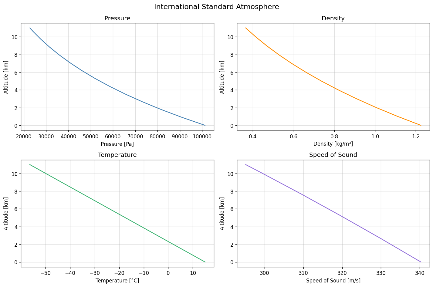
Sea-level pressure     : 101325.0 Pa
Sea-level temperature  : 15.00 °C
Sea-level speed of snd : 340.294 m/s
3. Airspeed conversions
pathsim_flight provides utility functions to convert between CAS, TAS, EAS, and Mach.
[3]:
cas_kts = 120.0  # Calibrated Airspeed [kts]

altitudes_ft = [0, 5000, 10000, 20000, 30000, 40000]

print(f"{'Altitude [ft]':>16} {'CAS [kts]':>10} {'TAS [kts]':>10} {'TAS/CAS':>8}")
print('-' * 50)
for alt_ft in altitudes_ft:
    alt_m = alt_ft * 0.3048
    p, rho, T, a = isa._eval(alt_m, 0.0)
    # CAS → TAS conversion (using sea-level standard density)
    rho_sl = 1.225  # kg/m³ sea-level standard
    tas_kts = cas_kts * (rho_sl / rho) ** 0.5
    print(f"{alt_ft:>16} {cas_kts:>10.1f} {tas_kts:>10.1f} {tas_kts/cas_kts:>8.3f}")
   Altitude [ft]  CAS [kts]  TAS [kts]  TAS/CAS
--------------------------------------------------
               0      120.0      120.0    1.000
            5000      120.0      129.3    1.077
           10000      120.0      139.6    1.164
           20000      120.0      164.3    1.370
           30000      120.0      196.0    1.634
           40000      120.0      241.4    2.012
4. JSBSimWrapper – embedding JSBSim in a PathSim diagram
JSBSimWrapper wraps a JSBSim FDM as a discrete-time Wrapper block.
Key parameters:
Parameter |
Description |
|---|---|
|
Discrete-time step for JSBSim [s] |
|
List of JSBSim property names for block inputs |
|
List of JSBSim property names for block outputs |
|
Aircraft directory name (e.g. |
|
KCAS for trim |
|
Altitude [ft] for trim |
Below we build a closed-loop pitch-hold autopilot using:
A
JSBSimWrapperfor the Cessna 172P dynamics.A
Constantblock to provide a pitch reference.A simple proportional controller (
Functionblock).
[4]:
from pathsim.blocks import Function, Amplifier, Adder

# ---------- Parameters ----------
AIRCRAFT     = 'c172p'
ALT_FT       = 5000.0    # trim altitude [ft]
AIRSPEED_KTS = 90.0      # trim KCAS
SIM_DUR      = 30.0      # simulation duration [s]
DT           = 1 / 60    # JSBSim time step [s]
Kp           = 0.5       # proportional gain [elevator/rad]
PITCH_REF    = 3.0       # pitch reference [deg]
# --------------------------------

# Flight dynamics model (JSBSim inside a PathSim block)
aircraft_block = JSBSimWrapper(
    T=DT,
    input_properties=['fcs/elevator-cmd-norm'],        # elevator input
    output_properties=[
        'attitude/theta-deg',     # pitch angle
        'position/h-sl-ft',       # altitude
        'velocities/vc-kts',      # calibrated airspeed
        'aero/alpha-deg',         # angle of attack
    ],
    aircraft_model=AIRCRAFT,
    trim_airspeed=AIRSPEED_KTS,
    trim_altitude=ALT_FT,
    trim_gamma=0.0,
)

# Reference pitch angle
pitch_ref = Constant(PITCH_REF)                        # deg

# Error = reference − actual pitch
pitch_error = Adder('+-')

# Proportional controller: elevator = Kp * error (deg → normalised)
controller = Amplifier(Kp / 90.0)    # /90 to stay roughly in [-1, 1]

# Record pitch, altitude, and airspeed
scope_flight = Scope(labels=['pitch_deg', 'alt_ft', 'vc_kts', 'alpha_deg'])
scope_ctrl   = Scope(labels=['elevator_cmd', 'pitch_error'])

sim_ap = Simulation(
    blocks=[pitch_ref, aircraft_block, pitch_error, controller, scope_flight, scope_ctrl],
    connections=[
        # Autopilot loop
        Connection(pitch_ref, pitch_error, scope_ctrl[1]),      # reference → error adder
        Connection(aircraft_block[0], pitch_error[1]),           # actual pitch → error adder
        Connection(pitch_error, controller, scope_ctrl[0]),      # error → gain
        Connection(controller, aircraft_block),                  # elevator command → FDM
        # Scopes
        Connection(aircraft_block[0], scope_flight[0]),          # pitch
        Connection(aircraft_block[1], scope_flight[1]),          # altitude
        Connection(aircraft_block[2], scope_flight[2]),          # airspeed
        Connection(aircraft_block[3], scope_flight[3]),          # AoA
    ],
    dt=DT
)

sim_ap.run(SIM_DUR)

print("Autopilot simulation complete")
11:44:06 - INFO - LOGGING (log: True)
11:44:06 - INFO - BLOCKS (total: 6, dynamic: 0, static: 6, eventful: 1)
11:44:06 - INFO - GRAPH (nodes: 6, edges: 10, alg. depth: 1, loop depth: 3, runtime: 0.125ms)
11:44:06 - INFO - STARTING -> TRANSIENT (Duration: 30.00s)
11:44:06 - INFO - --------------------   1% | 0.0s<0.2s | 7734.5 it/s
11:44:06 - INFO - ####----------------  20% | 0.0s<0.1s | 11297.0 it/s
11:44:06 - INFO - ########------------  40% | 0.1s<0.2s | 6882.7 it/s
11:44:06 - INFO - ############--------  60% | 0.2s<0.1s | 11915.5 it/s
11:44:06 - INFO - ################----  80% | 0.2s<0.0s | 11143.1 it/s
11:44:06 - INFO - #################### 100% | 0.3s<--:-- | 10241.3 it/s
11:44:06 - INFO - FINISHED -> TRANSIENT (total steps: 1801, successful: 1801, runtime: 270.96 ms)
Autopilot simulation complete
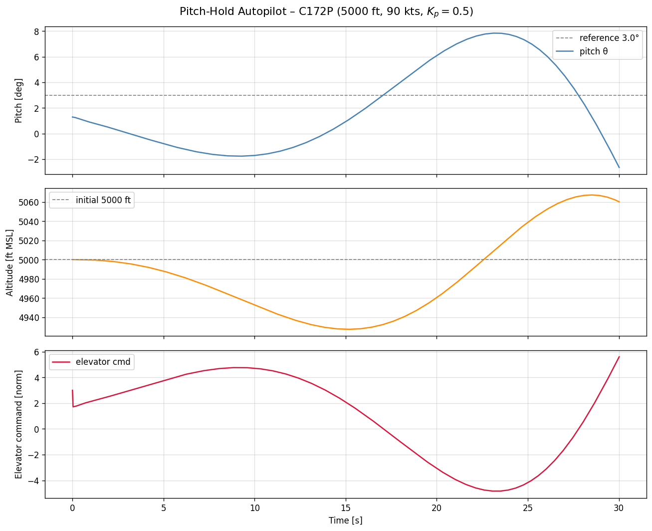
5. Plot the results
[5]:
t_ap, flight_data = scope_flight.read()
pitch_ap, alt_ap, vc_ap, aoa_ap = flight_data[0], flight_data[1], flight_data[2], flight_data[3]
t_ctrl, ctrl_data = scope_ctrl.read()
elev_ap, err_ap = ctrl_data[0], ctrl_data[1]

fig, axes = plt.subplots(3, 1, figsize=(11, 9), sharex=True)
fig.suptitle(
    f'Pitch-Hold Autopilot – {AIRCRAFT.upper()} '
    f'({ALT_FT:.0f} ft, {AIRSPEED_KTS:.0f} kts, $K_p={Kp}$)',
    fontsize=13
)

axes[0].axhline(PITCH_REF, color='grey', linestyle='--', linewidth=1.0,
                label=f'reference {PITCH_REF}°')
axes[0].plot(t_ap, pitch_ap, color='steelblue', linewidth=1.5, label='pitch θ')
axes[0].set_ylabel('Pitch [deg]')
axes[0].legend()

axes[1].plot(t_ap, alt_ap, color='darkorange', linewidth=1.5)
axes[1].axhline(ALT_FT, color='grey', linestyle='--', linewidth=1.0, label=f'initial {ALT_FT:.0f} ft')
axes[1].set_ylabel('Altitude [ft MSL]')
axes[1].legend()

axes[2].plot(t_ctrl, elev_ap, color='crimson', linewidth=1.5, label='elevator cmd')
axes[2].set_ylabel('Elevator command [norm]')
axes[2].set_xlabel('Time [s]')
axes[2].legend()

plt.tight_layout()
plt.savefig('autopilot_pitch_hold.png', bbox_inches='tight')
plt.show()
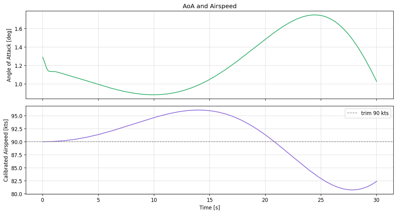
6. Angle-of-attack and airspeed
[6]:
fig, axes = plt.subplots(2, 1, figsize=(11, 6), sharex=True)

axes[0].plot(t_ap, aoa_ap, color='mediumseagreen', linewidth=1.5)
axes[0].set_ylabel('Angle of Attack [deg]')
axes[0].set_title('AoA and Airspeed')

axes[1].plot(t_ap, vc_ap, color='mediumpurple', linewidth=1.5)
axes[1].axhline(AIRSPEED_KTS, color='grey', linestyle='--', linewidth=1.0,
                label=f'trim {AIRSPEED_KTS:.0f} kts')
axes[1].set_ylabel('Calibrated Airspeed [kts]')
axes[1].set_xlabel('Time [s]')
axes[1].legend()

plt.tight_layout()
plt.savefig('autopilot_aoa_airspeed.png', bbox_inches='tight')
plt.show()