Airfoil Geometry and Aerodynamics

Level: Beginner

This notebook introduces NACA airfoil geometry and fundamental airfoil aerodynamics using thin-airfoil theory.

Topics covered

• NACA 4-digit and 5-digit airfoil geometry generation

• Airfoil coordinate visualization

• Thickness and camber distributions

• Lift coefficient vs. angle of attack (thin-airfoil theory)

• Effect of camber and thickness on aerodynamic performance

Prerequisites

• Basic Python and NumPy familiarity

• Elementary aerodynamics concepts (lift, drag, angle of attack)

References

• Abbott, I.H., and Von Doenhoff, A.E., Theory of Wing Sections, Dover, 1959

• Anderson, J.D., Introduction to Flight, McGraw-Hill, 2016

# Standard library imports
import numpy as np
import matplotlib.pyplot as plt
import matplotlib.gridspec as gridspec
import sys
import os

print("Setting up environment...")
print(f"Current working directory: {os.getcwd()}")

# Resolve project root from this notebook location and add src/ to import path
notebook_dir = os.getcwd()
project_root = os.path.abspath(os.path.join(notebook_dir, "..", ".."))
src_root = os.path.join(project_root, "src")

print(f"Resolved project root: {project_root}")
if not os.path.isdir(src_root):
    raise FileNotFoundError(f"Could not find src directory at: {src_root}")

if src_root not in sys.path:
    sys.path.insert(0, src_root)

print(f"Using src path: {src_root}")
from aerodemo.naca_airfoil import NACAFourDigit, NACAFiveDigit

# Matplotlib style
plt.rcParams.update({
    'figure.dpi': 100,
    'axes.grid': True,
    'grid.alpha': 0.3,
    'font.size': 11,
})
print("Setup complete.")

Setting up environment...
Current working directory: f:\agodemar\AeroDemonstrator\notebooks\01_airfoil
Resolved project root: f:\agodemar\AeroDemonstrator
Using src path: f:\agodemar\AeroDemonstrator\src
Setup complete.

1. NACA 4-Digit Airfoil Geometry

The NACA 4-digit series is defined by:

• 1st digit: maximum camber \(m\) as percentage of chord (0–9%)

• 2nd digit: location of maximum camber \(p\) in tenths of chord (0–9)

• Last 2 digits: maximum thickness \(t\) as percentage of chord

For example, NACA 2412 has:

• \(m = 0.02\) (2% camber)

• \(p = 0.4\) (camber at 40% chord)

• \(t = 0.12\) (12% thick)

The thickness distribution formula (Abbott & Von Doenhoff) is:

\[y_t = \frac{t}{0.2}\left(0.2969\sqrt{x} - 0.1260 x - 0.3516 x^2 + 0.2843 x^3 - 0.1015 x^4\right)\]

# --- Generate a family of NACA 4-digit airfoils ---
designations_4digit = ['0006', '0009', '0012', '2412', '4412', '2415']

fig, axes = plt.subplots(2, 3, figsize=(14, 7))
axes = axes.flatten()

for ax, des in zip(axes, designations_4digit):
    af = NACAFourDigit(des, n_points=200)
    xu, yu, xl, yl = af.coordinates()

    ax.plot(xu, yu, 'b-', linewidth=1.5, label='Upper surface')
    ax.plot(xl, yl, 'r-', linewidth=1.5, label='Lower surface')
    ax.fill_between(xu, yu, xl, alpha=0.08, color='steelblue')
    ax.set_aspect('equal')
    ax.set_title(f'NACA {des}', fontsize=12, fontweight='bold')
    ax.set_xlabel('x/c')
    ax.set_ylabel('y/c')
    ax.set_xlim(-0.05, 1.05)
    ax.legend(fontsize=8, loc='upper right')

plt.suptitle('NACA 4-Digit Airfoil Family', fontsize=14, fontweight='bold', y=1.01)
plt.tight_layout()
plt.savefig('naca4digit_family.png', bbox_inches='tight', dpi=100)
plt.show()
print("Figure saved as naca4digit_family.png")

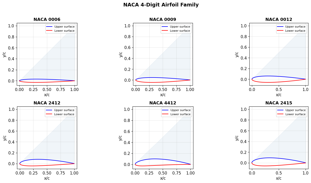
Figure saved as naca4digit_family.png

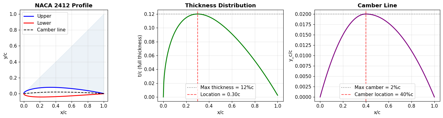
2. Thickness and Camber Distributions

Let us examine how thickness and camber vary along the chord for NACA 2412.

af_2412 = NACAFourDigit('2412', n_points=300)
x = np.linspace(0, 1, 300)

yt = af_2412.thickness(x)
yc, dyc_dx = af_2412.camber_line(x)

xu, yu, xl, yl = af_2412.coordinates()

fig, axes = plt.subplots(1, 3, figsize=(15, 4))

# Airfoil shape
ax = axes[0]
ax.plot(xu, yu, 'b-', linewidth=2, label='Upper')
ax.plot(xl, yl, 'r-', linewidth=2, label='Lower')
ax.plot(x, yc, 'k--', linewidth=1.5, label='Camber line')
ax.fill_between(xu, yu, xl, alpha=0.1, color='steelblue')
ax.set_aspect('equal')
ax.set_title('NACA 2412 Profile', fontweight='bold')
ax.set_xlabel('x/c')
ax.set_ylabel('y/c')
ax.legend()

# Thickness distribution
ax = axes[1]
ax.plot(x, yt * 2, 'g-', linewidth=2)
ax.axhline(af_2412.t, color='k', linestyle=':', alpha=0.5,
           label=f'Max thickness = {af_2412.t*100:.0f}%c')
idx_max = np.argmax(yt)
ax.axvline(x[idx_max], color='r', linestyle='--', alpha=0.7,
           label=f'Location = {x[idx_max]:.2f}c')
ax.set_title('Thickness Distribution', fontweight='bold')
ax.set_xlabel('x/c')
ax.set_ylabel('t/c (full thickness)')
ax.legend()

# Camber line
ax = axes[2]
ax.plot(x, yc, 'purple', linewidth=2)
ax.axhline(af_2412.m, color='k', linestyle=':', alpha=0.5,
           label=f'Max camber = {af_2412.m*100:.0f}%c')
ax.axvline(af_2412.p, color='r', linestyle='--', alpha=0.7,
           label=f'Camber location = {af_2412.p*100:.0f}%c')
ax.set_title('Camber Line', fontweight='bold')
ax.set_xlabel('x/c')
ax.set_ylabel('y_c/c')
ax.legend()

plt.tight_layout()
plt.savefig('naca2412_analysis.png', bbox_inches='tight', dpi=100)
plt.show()

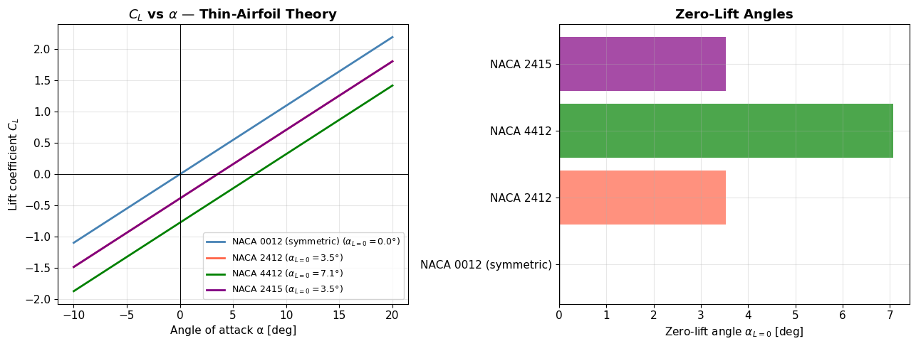
3. Thin-Airfoil Theory: Lift vs. Angle of Attack

Thin-airfoil theory gives the lift coefficient as:

\[C_L = 2\pi(\alpha - \alpha_{L=0})\]

where \(\alpha_{L=0}\) is the zero-lift angle of attack, which depends on the camber.

For symmetric airfoils (\(m=0\)), \(\alpha_{L=0} = 0\). For cambered airfoils, \(\alpha_{L=0} < 0\) (lift at zero geometric angle of attack).

airfoils_compare = {
    'NACA 0012 (symmetric)': NACAFourDigit('0012'),
    'NACA 2412': NACAFourDigit('2412'),
    'NACA 4412': NACAFourDigit('4412'),
    'NACA 2415': NACAFourDigit('2415'),
}

alpha_range = np.linspace(-10, 20, 100)

fig, axes = plt.subplots(1, 2, figsize=(13, 5))

colors = ['steelblue', 'tomato', 'green', 'purple']

# CL vs alpha
ax = axes[0]
for (name, af), color in zip(airfoils_compare.items(), colors):
    CL = [af.cl(a) for a in alpha_range]
    al0 = np.rad2deg(af.zero_lift_angle())
    ax.plot(alpha_range, CL, color=color, linewidth=2,
            label=f'{name} ($\\alpha_{{L=0}}={al0:.1f}°$)')
ax.axhline(0, color='k', linewidth=0.7)
ax.axvline(0, color='k', linewidth=0.7)
ax.set_xlabel('Angle of attack α [deg]')
ax.set_ylabel('Lift coefficient $C_L$')
ax.set_title('$C_L$ vs $\\alpha$ — Thin-Airfoil Theory', fontweight='bold')
ax.legend(fontsize=9)

# Zero-lift angles bar chart
ax = axes[1]
names = list(airfoils_compare.keys())
al0_values = [np.rad2deg(af.zero_lift_angle()) for af in airfoils_compare.values()]
ax.barh(names, al0_values, color=colors, alpha=0.7)
ax.axvline(0, color='k', linewidth=1)
ax.set_xlabel('Zero-lift angle $\\alpha_{L=0}$ [deg]')
ax.set_title('Zero-Lift Angles', fontweight='bold')

plt.tight_layout()
plt.savefig('cl_vs_alpha.png', bbox_inches='tight', dpi=100)
plt.show()

# Print summary
print("\nAirfoil Properties Summary:")
print(f"{'Airfoil':<20} {'m':>6} {'p':>6} {'t':>6} {'α_L0 [°]':>10}")
print("-" * 50)
for name, af in airfoils_compare.items():
    al0_deg = np.rad2deg(af.zero_lift_angle())
    label = name.split()[1]
    print(f"NACA {label:<16} {af.m*100:>5.1f}% {af.p*100:>5.0f}% {af.t*100:>5.0f}% {al0_deg:>10.2f}")

Airfoil Properties Summary:
Airfoil                   m      p      t   α_L0 [°]
--------------------------------------------------
NACA 0012               0.0%     0%    12%       0.00
NACA 2412               2.0%    40%    12%       3.53
NACA 4412               4.0%    40%    12%       7.06
NACA 2415               2.0%    40%    15%       3.53

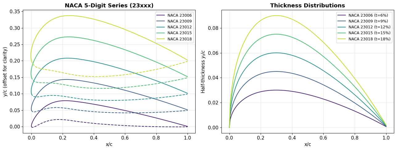
4. NACA 5-Digit Airfoils

The NACA 5-digit series provides higher design lift coefficients for the same thickness. Common examples: 23012, 23015, 23018.

The first three digits encode the design lift coefficient and camber line type.

designations_5digit = ['23006', '23009', '23012', '23015', '23018']
colors5 = plt.cm.viridis(np.linspace(0.1, 0.9, len(designations_5digit)))

fig, axes = plt.subplots(1, 2, figsize=(13, 5))

# Profile shapes (offset vertically for clarity)
ax = axes[0]
for i, des in enumerate(designations_5digit):
    af = NACAFiveDigit(des)
    xu, yu, xl, yl = af.coordinates()
    offset = i * 0.05
    ax.plot(xu, yu + offset, color=colors5[i], linewidth=1.5, label=f'NACA {des}')
    ax.plot(xl, yl + offset, color=colors5[i], linewidth=1.5, linestyle='--')
ax.set_xlabel('x/c')
ax.set_ylabel('y/c (offset for clarity)')
ax.set_title('NACA 5-Digit Series (23xxx)', fontweight='bold')
ax.legend(fontsize=9)

# Thickness as function of last two digits
ax = axes[1]
thicknesses = [int(des[3:]) for des in designations_5digit]
for i, des in enumerate(designations_5digit):
    af = NACAFiveDigit(des)
    x_pts = np.linspace(0, 1, 200)
    yt = af.thickness(x_pts)
    ax.plot(x_pts, yt, color=colors5[i], linewidth=1.5, label=f'NACA {des} (t={af.t*100:.0f}%)')
ax.set_xlabel('x/c')
ax.set_ylabel('Half-thickness $y_t/c$')
ax.set_title('Thickness Distributions', fontweight='bold')
ax.legend(fontsize=9)

plt.tight_layout()
plt.savefig('naca5digit_family.png', bbox_inches='tight', dpi=100)
plt.show()

5. Summary

In this notebook we have:

1. Generated NACA 4-digit airfoil coordinates using the standard thickness and camber formulas

2. Visualized the airfoil family, thickness and camber distributions

3. Applied thin-airfoil theory to compute lift curves

4. Compared cambered vs. symmetric airfoils

5. Introduced NACA 5-digit series

Key takeaways

• Camber shifts the lift curve to the left (negative \(\alpha_{L=0}\))

• All thin airfoils have the same lift-curve slope: \(2\pi\) per radian ≈ \(0.1097\) per degree

• Thickness does not affect lift in thin-airfoil theory (but affects stall)

Next steps

Proceed to ../02_finite_wing/finite_wing_vlm.ipynb to study finite wing effects.